
")
Summary
The goal of this blog is to show how customers can train a transformer model from scratch using open source Python libraries on Nutanix Cloud Platform (NCP). Transformer, which is the core model architecture of ChatGPT, is one of the most prominent deep learning models in the contemporary era [1]. Transformer is a remarkable neural network architecture because it is a general-purpose differentiable computing machine. It is expressive in the forward pass with multiple layers, dimensions, heads, and modalities; optimizable via back-propagation, gradient descent, and other mathematical techniques; and finally computationally efficient through high parallelism. In fact, all Foundation models—such as large language models like LLaMA, Universal Speech Model, and other generative AI models like Stable Diffusion use different variants of the transformer architecture. Therefore, to compete in the age of AI, an enterprise needs to harness granular understanding of transformer architecture. In this blog, we delve into the implementation of a transformer model for sequence memorization tasks to provide our users with much-needed insight into transformer architecture, while showing them the simplicity of our platform for the cutting-edge AI/ML workloads.
Use Cases for Nutanix
Transformers has revolutionized the trajectory of modern AI/ML applications with its superior performance and parallelizability. A transformer model is useful in many important enterprise applications such as:
- Visual perception (e.g., optical character recognition, object detection)
- Automated chatbot (e.g., ChatGPT and numerous variants)
- Speech recognition systems (e.g., Siri, Alexa, Google assistant)
- Retail (e.g. Amazon Go)
Therefore, it is critical that our customers understand the basic mechanisms of training a transformer model and also have the ability of training transformer models from scratch on a Nutanix cluster. Training from scratch helps in deeper understanding which facilitates a whole gamut of MLOPs tasks including data engineering, feature engineering, compute resource planning, hyperparameter tuning, rapid prototyping, and better life cycle management.
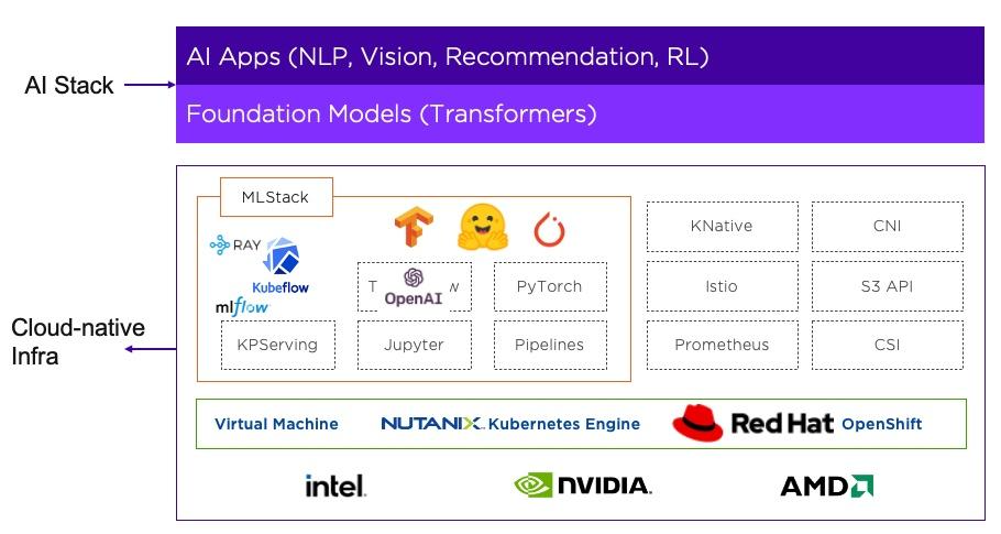
Figure 1 shows how AI/ML is being integrated into the core Nutanix infrastructure layer. The foundation models based on transformer architecture, such as BERT, GPT-3, DALL-E, assume a central role in this integration. We ensure customers can build a wide array of AI apps such as NLP, vision, contact center, recommendation, etc. by empowering them with the capability of transformer model training from scratch.
Introduction
Foundation models, such as GPT-3, BERT, DALL-E, have captivated human/societal attention and have accelerated the enterprise AI adoption. At its core, it is a transformer model which is both high-performance and low-overhead. It dispenses the need for recurrent neural networks (RNNs), long short-term memory (LSTM), and convolution neural networks (CNNs) in sequence modeling. Before we deep dive into transformer training, we will briefly touch upon the supporting Nutanix Cloud Platform (NCP).
Setting up Nutanix Cloud Platform for Transformer Model Training
At Nutanix, we are dedicated to enable customers with the ability to build and deploy intelligent applications anywhere—edge, core data centers, service provider infrastructure, and public clouds. Prism Element1 (PE) is a service built into the platform for every Nutanix cluster deployed. Prism Element enables a user to fully configure, manage, and monitor Nutanix clusters running any hypervisor. Therefore, the first step of the Nutanix infrastructure setup is to log into a Prism Element, as Shown in Figure 2.
- Log into a Prism Element (the UI is shown in Figure 2)

- Set up the VM
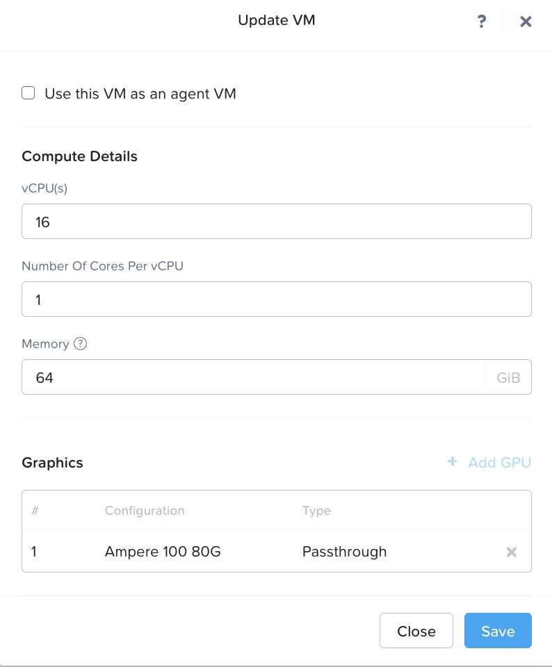
On the Prism Element we log in, we set up a VM, hosted on Nutanix AHV hypervisor. As shown in Figure 3, the VM has following resource configuration settings:
- Ubuntu Linux 22.04 operating system
- 16 single core vCPUs
- 64 GB of RAM
- NVIDIA A1002 tensor core passthrough GPU with 80GB memory
The GPU is installed with the NVIDIA RTX 15.0 driver for Ubuntu OS (NVIDIA-Linux-x86_64-525.60.13-grid.run). The large deep learning models with transformer architecture require GPU or other compute accelerators with high memory bandwidth, large registers and L1 memory.
- Underlying A100 GPU
NVIDIA A100 Tensor Core GPU is designed to power the world’s highest-performing elastic data centers for AI, data analytics, and HPC. Powered by the NVIDIA Ampere Architecture3, A100 is the engine of the NVIDIA data center platform. A100 provides up to 20X higher performance over the prior generation and can be partitioned into seven GPU instances to dynamically adjust to shifting demands. The A100 80GB debuts the world’s fastest memory bandwidth at over 2 terabytes per second (TB/s) to run the largest models and datasets. To peek into the detailed features of A100 GPU, we run nvidia-smi4 command which is a command line utility, based on top of the NVIDIA Management Library (NVML), intended to aid in the management and monitoring of NVIDIA GPU devices. The output of the nvidia-smi command is shown in Table 1. It shows the Driver Version to be 525.60.13 and CUDA5 version to be 12.0.
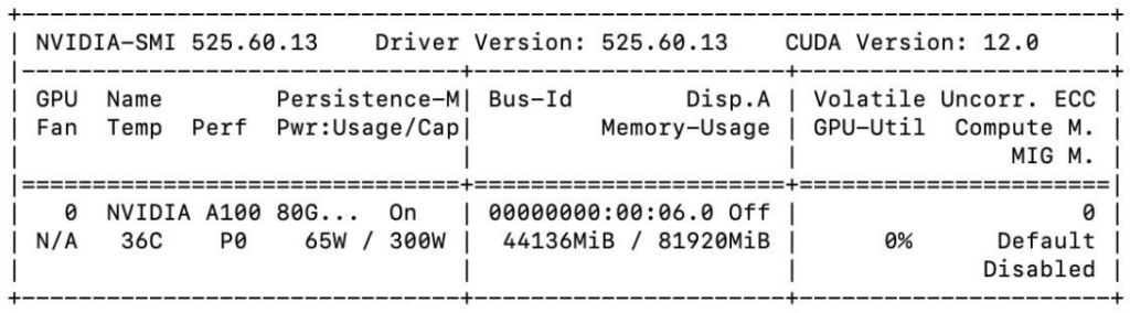
Table 1 shows several critical features of the A100 GPU we used. The details of these features are described in Table 2.
| Feature | Value | Description |
|---|---|---|
| GPU | 0 | GPU Index |
| Name | NVIDIA A100 | GPU Name |
| Temp | 36 C | Core GPU Temperature |
| Perf | P0 | GPU Performance |
| Persistence-M | On | Persistence Mode |
| Pwr: Usage/Cap | 65 W / 300 W | GPU Power Usage and it capability |
| Bus Id | 00000000:00:06.0 | domain:bus:device.function |
| Disp. A | Off | Display Active |
| Memory-Usage | 44136MiB / 81920MiB | Memory allocation out of total memory |
| Volatile Uncorr. ECC | 0 | Counter of uncorrectable ECC memory error |
| GPU-Util | 0% | GPU Utilization |
| Compute M. | Default | Compute Mode |
| MIG M. | Disabled | Multi-Instance Mode |
Transformer Training on Nutanix Cloud Platform
In this blog, we will train a transformer model for the task of sequence memorization.
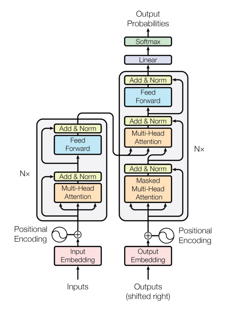
We train this transformer model purely with standard open source libraries predominantly PyTorch 2.06 . Figure 4 shows the architecture of a transformer model. The Transformer follows an encoder-decoder architecture using stacked self-attention and point-wise, fully connected layers for both the encoder and the decoder blocks, shown in the left and right halves of Figure 4, respectively. The model has 65M parameters, 6 layers, 512 dimensions, 8 heads, sequence length of 10, and a variable learning schedule.
Implementation of the Encoder
The encoder (the left half of Figure 4) takes an input sequence and maps into an intermediate representation. Here we use a stack of N layers. It also uses layer normalization (LayerNorm) which is a technique to normalize the distributions of intermediate layers. It prompts smoother gradients, faster training, and better generalization accuracy [1].
Code Block 1: Encoder Implementation
class Encoder(nn.Module):
   "Core encoder is a stack of N layers"


   def __init__(self, layer, N):
       super(Encoder, self).__init__()
       self.layers = clones(layer, N)
       self.norm = LayerNorm(layer.size)


   def forward(self, x, mask):
       "Pass the input (and mask) through each layer in turn."
       for layer in self.layers:
           x = layer(x, mask)
       return self.norm(x)
Each layer in the encoder network has two sub-layers. The first is a multi-head self-attention mechanism, and the second is a simple, position-wise fully connected feed-forward network. Code Block 2 shows the implementation of an Encode Layer.
Code Block 2: Encode Layer Implementation
class EncoderLayer(nn.Module):
   "Encoder is made up of self-attn and feed forward (defined below)"


   def __init__(self, size, self_attn, feed_forward, dropout):
       super(EncoderLayer, self).__init__()
       self.self_attn = self_attn
       self.feed_forward = feed_forward
       self.sublayer = clones(SublayerConnection(size, dropout), 2)
       self.size = size


   def forward(self, x, mask):
       "Follow Figure 1 (left) for connections."
       x = self.sublayer[0](x, lambda x: self.self_attn(x, x, x, mask))
       return self.sublayer[1](x, self.feed_forward)
Implementation of the Decoder
The decoder (the right half of Fig 1) takes the intermediate representation from the encoder and generates an output sequence one element at a time. At each step the model is auto-regressive, consuming the previously generated symbols as additional input when generating the next. Code Block 3 shows the implementation of a Decoder.
Code Block 3: Decoder Implementation
class Decoder(nn.Module):
   "Generic N layer decoder with masking."


   def __init__(self, layer, N):
       super(Decoder, self).__init__()
       self.layers = clones(layer, N)
       self.norm = LayerNorm(layer.size)


   def forward(self, x, memory, src_mask, tgt_mask):
       for layer in self.layers:
           x = layer(x, memory, src_mask, tgt_mask)
       return self.norm(x)
Like the encoder layer, the decoder layer has two sublayers. Additionally, the decoder inserts a third sub-layer, which performs multi-head attention over the output of the encoder stack. Similar to the encoder, we employ residual connections around each of the sub-layers, followed by layer normalization.
Code Block 4: Decode Layer Implementation
Code Block 4 shows the implementation of a Decode Layer.
class DecoderLayer(nn.Module):
   "Decoder is made of self-attn, src-attn, and feed forward (defined below)"


   def __init__(self, size, self_attn, src_attn, feed_forward, dropout):
       super(DecoderLayer, self).__init__()
       self.size = size
       self.self_attn = self_attn
       self.src_attn = src_attn
       self.feed_forward = feed_forward
       self.sublayer = clones(SublayerConnection(size, dropout), 3)


   def forward(self, x, memory, src_mask, tgt_mask):
       "Follow Figure 1 (right) for connections."
       m = memory
       x = self.sublayer[0](x, lambda x: self.self_attn(x, x, x, tgt_mask))
       x = self.sublayer[1](x, lambda x: self.src_attn(x, m, m, src_mask))
       return self.sublayer[2](x, self.feed_forward)
Implementation of Attention
Evidently, attention is the key building block in a transformer model. We have covered the attention mechanism in detail on another dev article: Run Attention on Nutanix.
An attention function can be described as mapping a query and a set of key-value pairs to an output, where the query, keys, values, and output are all vectors. The output is computed as a weighted sum of the values, where the weight assigned to each value is computed by a compatibility function of the query with the corresponding key. Here is a formulation for the computation of attention function as a function of query (Q), key (K), and value (V). Here, dk is the dimension of key (K).
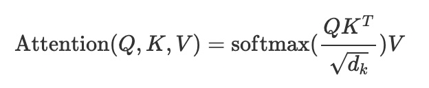
Code Block 5: Attention Function
def attention(query, key, value, mask=None, dropout=None):
   "Compute 'Scaled Dot Product Attention'"
   d_k = query.size(-1)
   scores = torch.matmul(query, key.transpose(-2, -1)) / math.sqrt(d_k)
   if mask is not None:
       scores = scores.masked_fill(mask == 0, -1e9)
   p_attn = scores.softmax(dim=-1)
   if dropout is not None:
       p_attn = dropout(p_attn)
   return torch.matmul(p_attn, value), p_attn
Instead of performing a single attention function with dk-dimensional keys, values and queries, we found it beneficial to linearly project the queries, keys and values h times with different, learned linear projections. On each of these projected versions of queries, keys and values, we then perform the attention function in parallel, yielding dv-dimensional output values. For further details, the reader is encouraged to review the seminal paper by Vaswani et al.: Attention is All You Need.
Code Block 6
class MultiHeadedAttention(nn.Module):
    def __init__(self, h, d_model, dropout=0.1):
       "Take in model size and number of heads."
       super(MultiHeadedAttention, self).__init__()
       assert d_model % h == 0
       # We assume d_v always equals d_k
       self.d_k = d_model // h
       self.h = h
       self.linears = clones(nn.Linear(d_model, d_model), 4)
       self.attn = None
       self.dropout = nn.Dropout(p=dropout)


    def forward(self, query, key, value, mask=None):
       "Implements Figure 2"
       if mask is not None:
           # Same mask applied to all h heads.
           mask = mask.unsqueeze(1)
       nbatches = query.size(0)


       # 1) Do all the linear projections in batch from d_model => h x d_k
       query, key, value = [
           lin(x).view(nbatches, -1, self.h, self.d_k).transpose(1, 2)
           for lin, x in zip(self.linears, (query, key, value))
       ]


       # 2) Apply attention on all the projected vectors in batch.
       x, self.attn = attention(
           query, key, value, mask=mask, dropout=self.dropout
       )


       # 3) "Concat" using a view and apply a final linear.
       x = (
           x.transpose(1, 2)
           .contiguous()
           .view(nbatches, -1, self.h * self.d_k)
       )
       del query
       del key
       del value
       return self.linears[-1](x)
Full Model
Our model is trained using the Adam optimizer with β1 = 0.9, β2 = 0.98 and 𝝐 = 10−9
We have a variable learning rate with this formula:
lr = d −0.5 model · min(step_num−0.5 , step_num · warmup_steps−1.5 )This corresponds to increasing the learning rate linearly for the first warmup_steps training steps, and decreasing it thereafter proportionally to the inverse square root of the step number. We used warmup_steps = 4000.
We use a transformer model with following architecture specifications: 6 different stacking layers, 8 head count, 512 output dimensions, 64 key and value dimensions.
Code Block 7
def make_model(
   src_vocab, tgt_vocab, N=6, d_model=512, d_ff=2048, h=8, dropout=0.1):
   "Helper: Construct a model from hyperparameters."
   c = copy.deepcopy
   attn = MultiHeadedAttention(h, d_model)
   ff = PositionwiseFeedForward(d_model, d_ff, dropout)
   position = PositionalEncoding(d_model, dropout)
   model = EncoderDecoder(
       Encoder(EncoderLayer(d_model, c(attn), c(ff), dropout), N),
       Decoder(DecoderLayer(d_model, c(attn), c(attn), c(ff), dropout), N),
       nn.Sequential(Embeddings(d_model, src_vocab), c(position)),
       nn.Sequential(Embeddings(d_model, tgt_vocab), c(position)),
       Generator(d_model, tgt_vocab),
   )


   # This was important from their code.
   # Initialize parameters with Glorot / fan_avg.
   for p in model.parameters():
       if p.dim() > 1:
           nn.init.xavier_uniform_(p)
   return model
Inference before Training
Here, we make a forward step to generate a prediction of the model. We use our transformer to memorize the input. As you will see the output is randomly generated due to the fact that the model is not trained yet. In the next tutorial we will build the training function and try to train our model to memorize the numbers from 1 to 10.
Code Block 8
def inference_test():
   test_model = make_model(11, 11, 2)
   test_model.eval()
   src = torch.LongTensor([[1, 2, 3, 4, 5, 6, 7, 8, 9, 10]])
   src_mask = torch.ones(1, 1, 10)


   memory = test_model.encode(src, src_mask)
   ys = torch.zeros(1, 1).type_as(src)


   for i in range(9):
       out = test_model.decode(
           memory, src_mask, ys, subsequent_mask(ys.size(1)).type_as(src.data)
       )
       prob = test_model.generator(out[:, -1])
       _, next_word = torch.max(prob, dim=1)
       next_word = next_word.data[0]
       ys = torch.cat(
           [ys, torch.empty(1, 1).type_as(src.data).fill_(next_word)], dim=1
       )


   print("Example Untrained Model Prediction:", ys)


def run_tests():
   for _ in range(10):
       inference_test()


show_example(run_tests)
As the model is untrained, the result is random.
Code Block 9: Untrained Model Output
Example Untrained Model Prediction: tensor([[0, 0, 0, 0, 0, 0, 0, 0, 0, 0]])
Example Untrained Model Prediction: tensor([[0, 3, 4, 4, 4, 4, 4, 4, 4, 4]])
Example Untrained Model Prediction: tensor([[ 0, 10, 10, 10,  3,  2,  5,  7,  9,  6]])
Example Untrained Model Prediction: tensor([[ 0,  4,  3,  6, 10, 10,  2,  6,  2,  2]])
Example Untrained Model Prediction: tensor([[ 0,  9,  0,  1,  5, 10,  1,  5, 10,  6]])
Example Untrained Model Prediction: tensor([[ 0,  1,  5,  1, 10,  1, 10, 10, 10, 10]])
Example Untrained Model Prediction: tensor([[ 0,  1, 10,  9,  9,  9,  9,  9,  1,  5]])
Example Untrained Model Prediction: tensor([[ 0,  3,  1,  5, 10, 10, 10, 10, 10, 10]])
Example Untrained Model Prediction: tensor([[ 0,  3,  5, 10,  5, 10,  4,  2,  4,  2]])
Example Untrained Model Prediction: tensor([[0, 5, 6, 2, 5, 6, 2, 6, 2, 2]])
Training Loop
Code Block 10: Invoke the training epoch
class TrainState:
   """Track number of steps, examples, and tokens processed"""


   step: int = 0  # Steps in the current epoch
   accum_step: int = 0  # Number of gradient accumulation steps
   samples: int = 0  # total # of examples used
   tokens: int = 0  # total # of tokens processed


def run_epoch(
   data_iter,
   model,
   loss_compute,
   optimizer,
   scheduler,
   mode="train",
   accum_iter=1,
   train_state=TrainState(),
):
   """Train a single epoch"""
   start = time.time()
   total_tokens = 0
   total_loss = 0
   tokens = 0
   n_accum = 0
   for i, batch in enumerate(data_iter):
       out = model.forward(
           batch.src, batch.tgt, batch.src_mask, batch.tgt_mask
       )
       loss, loss_node = loss_compute(out, batch.tgt_y, batch.ntokens)
       # loss_node = loss_node / accum_iter
       if mode == "train" or mode == "train+log":
           loss_node.backward()
           train_state.step += 1
           train_state.samples += batch.src.shape[0]
           train_state.tokens += batch.ntokens
           if i % accum_iter == 0:
               optimizer.step()
               optimizer.zero_grad(set_to_none=True)
               n_accum += 1
               train_state.accum_step += 1
           scheduler.step()


       total_loss += loss
       total_tokens += batch.ntokens
       tokens += batch.ntokens
       if i % 40 == 1 and (mode == "train" or mode == "train+log"):
           lr = optimizer.param_groups[0]["lr"]
           elapsed = time.time() - start
           print(
               (
                   "Epoch Step: %6d | Accumulation Step: %3d | Loss: %6.2f "
                   + "| Tokens / Sec: %7.1f | Learning Rate: %6.1e"
               )
               % (i, n_accum, loss / batch.ntokens, tokens / elapsed, lr)
           )
           start = time.time()
           tokens = 0
       del loss
       del loss_node
   return total_loss / total_tokens, train_state
Inference after Training
Here is a code block that shows how to call training on a task of sequence memorization and evaluate the model inference.
Code Block 11
def example_simple_model():
   V = 11
   criterion = LabelSmoothing(size=V, padding_idx=0, smoothing=0.0)
   model = make_model(V, V, N=2)


   optimizer = torch.optim.Adam(
       model.parameters(), lr=0.5, betas=(0.9, 0.98), eps=1e-9
   )
   lr_scheduler = LambdaLR(
       optimizer=optimizer,
       lr_lambda=lambda step: rate(
           step, model_size=model.src_embed[0].d_model, factor=1.0, warmup=400
       ),
   )


   batch_size = 80
   for epoch in range(20):
       model.train()
       run_epoch(
           data_gen(V, batch_size, 20),
           model,
           SimpleLossCompute(model.generator, criterion),
           optimizer,
           lr_scheduler,
           mode="train",
       )
       model.eval()
       run_epoch(
           data_gen(V, batch_size, 5),
           model,
           SimpleLossCompute(model.generator, criterion),
           DummyOptimizer(),
           DummyScheduler(),
           mode="eval",
       )[0]


   model.eval()
   src = torch.LongTensor([[0, 1, 2, 3, 4, 5, 6, 7, 8, 9]])
   max_len = src.shape[1]
   src_mask = torch.ones(1, 1, max_len)
   print(greedy_decode(model, src, src_mask, max_len=max_len, start_symbol=0))
Here is the model evaluation from the training run:
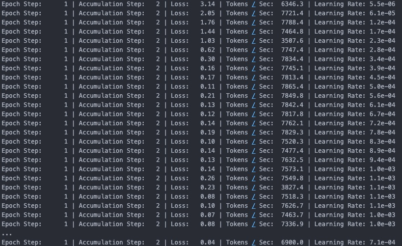
Code Block 12: Training Run Model Evaluation
We see the loss gradually reducing from 3.14 to 0.04 and learning rate varying between 5.5e-06 to 1.1e-03. One of the interesting statistics is tokens / sec which is the number of tokens processed in a single GPU per second. This number is important in rightsizing the supporting model infrastructure.
Here is the inference of the sequence memorization:
tensor([[0,1,2,3,4,5,6,7,8,9]])As we can see the model has successfully memorized the sequence: [0,1,2,…,9].
Carbon Footprint
Deep learning models, especially GPT type models, consume massive amounts of energy, responsible for carbon emissions. Therefore, it is important to be cognizant of the carbon footprints for deep learning model training. Based on a recent study (https://proceedings.mlsys.org/paper/2022/hash/ed3d2c21991e3bef5e069713af9fa6ca-Abstract.html) , the watt-hour consumed by a model:
Wh = GPU-h×(GPU power consumption)×PUEThe simple transformer model in this article for sequence memorization took 14 minutes in training on average. With a PUE of 1.1 and 65W GPU power consumption, the watt-hour for the model training:
Wh = (14/60) x 65 W x 1.1 = 16.7 WhWith the US national average carbon intensity factor of 0.385 kg CO2eq/KWh, we can use the following formula for the tons of carbon emissions:
tCO2eq = MWh × 0.385For the transformer model training in this blog the resulting carbon emission:
tCO2eq = 6.4 x 10⁻⁶ tonsAt Nutanix, we are dedicated to sustainable IT practices and continuously striving to reduce the carbon footprints for our customers.
Conclusion
We have shown how we can leverage our Nutanix Cloud Platform to train a transformer model for a simple sequence modeling task which is the heart of the current wave of generative AI, LLMs etc. Nutanix Cloud Platform allows customers to achieve consistency across their entire infrastructure stack, from edge to the cloud. In addition, we believe that Nutanix Cloud Platform can help customers with their ROI for cutting-edge AI workloads by a combination of class leading unified storage, better integrated management, operations and security, sustainability, along with data management and governance.
References
[1] Vaswani et al., “Attention is all you need“, NIPS 2017.
Appendix
Use Cases of Attention-based AI Models in the Industry
- Visual perception (e.g., optical character recognition, object detection).
- Automated chatbot (e.g., ChatGPT and numerous variants)
- Speech recognition systems (e.g., Siri, Alexa, Google assistant).
- Automated decision-making systems (e.g., AlphaGo)
- Robotics (e.g., retail packaging, manufacturing pipelines)
- Predictive healthcare (e.g., early disease recognition, AI driven protocols in cancer)
- Drug discovery (e.g., AlphaFold, high throughput docking)
- Compliance (e.g., named entity recognition, contract understanding)
- Legal (e.g., document summarization, compliance enforcement)
- Manufacturing (e.g., predictive maintenance tasks)
- Transportation (e.g., autonomous vehicle tasks)
- Developer productivity (e.g, code completion)
- Retail (e.g. reducing shrinkage, visual supply chain, fraud detection)
Footnotes
- https://portal.nutanix.com/page/documents/solutions/details?targetId=TN-2042-Prism:tn-executive-summary.html
- https://www.nvidia.com/en-us/data-center/a100/
- https://www.nvidia.com/en-us/data-center/ampere-architecture/
- https://developer.nvidia.com/nvidia-system-management-interface
- https://developer.nvidia.com/cuda-toolkit
- https://pytorch.org/get-started/pytorch-2.0/